Quantum Computing January 25, 2026 computer-science
Selected notes from COMS 4281 Introduction to Quantum Computing taught by Prof. Henry Yuen in Fall 2025.
Qubits
A quantum bit (or qubit) is the basic unit of information in quantum computing. Unlike classical bits that are exclusively 0 or 1, a qubit exists in a superposition of both states. However, upon measurement, the qubit collapses to a classical bit value.
Mathematically, a qubit state is represented as:
∣ ψ ⟩ = α ∣ 0 ⟩ + β ∣ 1 ⟩ |\psi\rangle = \alpha|0\rangle + \beta|1\rangle ∣ ψ ⟩ = α ∣0 ⟩ + β ∣1 ⟩ where α , β ∈ C \alpha, \beta \in \mathbb{C} α , β ∈ C ∣ α ∣ 2 + ∣ β ∣ 2 = 1 |\alpha|^2 + |\beta|^2 = 1 ∣ α ∣ 2 + ∣ β ∣ 2 = 1
The states ∣ 0 ⟩ |0\rangle ∣0 ⟩ ∣ 1 ⟩ |1\rangle ∣1 ⟩
∣ 0 ⟩ = ( 1 0 ) , ∣ 1 ⟩ = ( 0 1 ) |0\rangle = \begin{pmatrix} 1 \\ 0 \end{pmatrix}, \quad |1\rangle = \begin{pmatrix} 0 \\ 1 \end{pmatrix} ∣0 ⟩ = ( 1 0 ) , ∣1 ⟩ = ( 0 1 ) Systems and States
A quantum system S S S d d d ∣ 0 ⟩ , ∣ 1 ⟩ , … , ∣ d − 1 ⟩ |0\rangle, |1\rangle, \ldots, |d-1\rangle ∣0 ⟩ , ∣1 ⟩ , … , ∣ d − 1 ⟩
Mathematically : ∣ 0 ⟩ |0\rangle ∣0 ⟩ [ 1 , 0 , … ] T [1, 0, \ldots]^T [ 1 , 0 , … ] T Transformations : A system may undergo a transformation R R R R ∣ x ⟩ R|x\rangle R ∣ x ⟩
Mathematically, R R R
Composition: U R ∣ x ⟩ UR|x\rangle U R ∣ x ⟩ R R R U U U
Reversibility : In quantum computing, all transformations R R R reversible , i.e., R − 1 R^{-1} R − 1 R R − 1 = I RR^{-1} = I R R − 1 = I
Composite Systems
Composite systems are formed from two or more individual systems. If systems S 1 S_1 S 1 S 2 S_2 S 2 S 1 ⊗ S 2 S_1 \otimes S_2 S 1 ⊗ S 2
The state of the composite system is:
∣ x 1 ⟩ ⊗ ∣ x 2 ⟩ |x_1\rangle \otimes |x_2\rangle ∣ x 1 ⟩ ⊗ ∣ x 2 ⟩ This is often abbreviated as:
∣ x 1 ⟩ ⊗ ∣ x 2 ⟩ = ∣ x 1 ⟩ ∣ x 2 ⟩ = ∣ x 1 , x 2 ⟩ = ∣ x 1 x 2 ⟩ |x_1\rangle \otimes |x_2\rangle = |x_1\rangle|x_2\rangle = |x_1, x_2\rangle = |x_1 x_2\rangle ∣ x 1 ⟩ ⊗ ∣ x 2 ⟩ = ∣ x 1 ⟩ ∣ x 2 ⟩ = ∣ x 1 , x 2 ⟩ = ∣ x 1 x 2 ⟩ Transformations on composite systems : If R R R S 1 S_1 S 1 U U U S 2 S_2 S 2
( R ⊗ U ) ( ∣ x 1 ⟩ ⊗ ∣ x 2 ⟩ ) = R ∣ x 1 ⟩ ⊗ U ∣ x 2 ⟩ (R \otimes U)(|x_1\rangle \otimes |x_2\rangle) = R|x_1\rangle \otimes U|x_2\rangle ( R ⊗ U ) ( ∣ x 1 ⟩ ⊗ ∣ x 2 ⟩) = R ∣ x 1 ⟩ ⊗ U ∣ x 2 ⟩ Some transformations cannot be written as independent transformations on each subsystem. These are entangling operations , such as CNOT.
Measurement
When a qubit in state ∣ ψ ⟩ = α ∣ 0 ⟩ + β ∣ 1 ⟩ |\psi\rangle = \alpha|0\rangle + \beta|1\rangle ∣ ψ ⟩ = α ∣0 ⟩ + β ∣1 ⟩
Outcome ∣ 0 ⟩ |0\rangle ∣0 ⟩ ∣ α ∣ 2 |\alpha|^2 ∣ α ∣ 2
Outcome ∣ 1 ⟩ |1\rangle ∣1 ⟩ ∣ β ∣ 2 |\beta|^2 ∣ β ∣ 2
The state collapses to the measured outcome
Common Quantum Gates
Single-Qubit Gates
Pauli-X (NOT gate) :
X = ( 0 1 1 0 ) X = \begin{pmatrix} 0 & 1 \\ 1 & 0 \end{pmatrix} X = ( 0 1 1 0 ) Effect: X ∣ 0 ⟩ = ∣ 1 ⟩ X|0\rangle = |1\rangle X ∣0 ⟩ = ∣1 ⟩ X ∣ 1 ⟩ = ∣ 0 ⟩ X|1\rangle = |0\rangle X ∣1 ⟩ = ∣0 ⟩
Pauli-Z :
Z = ( 1 0 0 − 1 ) Z = \begin{pmatrix} 1 & 0 \\ 0 & -1 \end{pmatrix} Z = ( 1 0 0 − 1 ) Effect: Z ∣ 0 ⟩ = ∣ 0 ⟩ Z|0\rangle = |0\rangle Z ∣0 ⟩ = ∣0 ⟩ Z ∣ 1 ⟩ = − ∣ 1 ⟩ Z|1\rangle = -|1\rangle Z ∣1 ⟩ = − ∣1 ⟩
Hadamard (H) :
H = 1 2 ( 1 1 1 − 1 ) H = \frac{1}{\sqrt{2}}\begin{pmatrix} 1 & 1 \\ 1 & -1 \end{pmatrix} H = 2 1 ( 1 1 1 − 1 ) The Hadamard gate creates superposition:
H ∣ 0 ⟩ = 1 2 ( ∣ 0 ⟩ + ∣ 1 ⟩ ) = ∣ + ⟩ H ∣ 1 ⟩ = 1 2 ( ∣ 0 ⟩ − ∣ 1 ⟩ ) = ∣ − ⟩ \begin{align*}
H|0\rangle &= \frac{1}{\sqrt{2}}(|0\rangle + |1\rangle) = |+\rangle \\
H|1\rangle &= \frac{1}{\sqrt{2}}(|0\rangle - |1\rangle) = |-\rangle
\end{align*} H ∣0 ⟩ H ∣1 ⟩ = 2 1 ( ∣0 ⟩ + ∣1 ⟩) = ∣ + ⟩ = 2 1 ( ∣0 ⟩ − ∣1 ⟩) = ∣ − ⟩ General formula:
H ∣ a ⟩ = 1 2 ∑ b ∈ { 0 , 1 } ( − 1 ) a ⋅ b ∣ b ⟩ H|a\rangle = \frac{1}{\sqrt{2}}\sum_{b \in \{0,1\}} (-1)^{a\cdot b}|b\rangle H ∣ a ⟩ = 2 1 b ∈ { 0 , 1 } ∑ ( − 1 ) a ⋅ b ∣ b ⟩ Two-Qubit Gates
CNOT (Controlled-NOT) :
CNOT = ( 1 0 0 0 0 1 0 0 0 0 0 1 0 0 1 0 ) \text{CNOT} = \begin{pmatrix} 1 & 0 & 0 & 0 \\ 0 & 1 & 0 & 0 \\ 0 & 0 & 0 & 1 \\ 0 & 0 & 1 & 0 \end{pmatrix} CNOT = 1 0 0 0 0 1 0 0 0 0 0 1 0 0 1 0 Effect: Flips the target qubit if the control qubit is ∣ 1 ⟩ |1\rangle ∣1 ⟩
CNOT ∣ 00 ⟩ = ∣ 00 ⟩ \text{CNOT}|00\rangle = |00\rangle CNOT ∣00 ⟩ = ∣00 ⟩ CNOT ∣ 01 ⟩ = ∣ 01 ⟩ \text{CNOT}|01\rangle = |01\rangle CNOT ∣01 ⟩ = ∣01 ⟩ CNOT ∣ 10 ⟩ = ∣ 11 ⟩ \text{CNOT}|10\rangle = |11\rangle CNOT ∣10 ⟩ = ∣11 ⟩ CNOT ∣ 11 ⟩ = ∣ 10 ⟩ \text{CNOT}|11\rangle = |10\rangle CNOT ∣11 ⟩ = ∣10 ⟩
Partial Measurements in Non-Standard Bases
Measuring in Different Bases
Given a state ∣ ψ ⟩ = ∑ i , j α i j ∣ i ⟩ ∣ j ⟩ |\psi\rangle = \sum_{i,j} \alpha_{ij}|i\rangle|j\rangle ∣ ψ ⟩ = ∑ i , j α ij ∣ i ⟩ ∣ j ⟩ B = { ∣ b 0 ⟩ , ∣ b 1 ⟩ , … , ∣ b d ⟩ } B = \{|b_0\rangle, |b_1\rangle, \ldots, |b_d\rangle\} B = { ∣ b 0 ⟩ , ∣ b 1 ⟩ , … , ∣ b d ⟩}
The projection onto ∣ b ℓ ⟩ |b_\ell\rangle ∣ b ℓ ⟩
∣ v ℓ ⟩ = ( ∣ b ℓ ⟩ ⟨ b ℓ ∣ ⊗ I ) ∣ ψ ⟩ = ∑ i , j α i j ⟨ b ℓ ∣ i ⟩ ∣ b ℓ ⟩ ⊗ ∣ j ⟩ |v_\ell\rangle = (|b_\ell\rangle\langle b_\ell| \otimes I)|\psi\rangle = \sum_{i,j} \alpha_{ij}\langle b_\ell|i\rangle |b_\ell\rangle \otimes |j\rangle ∣ v ℓ ⟩ = ( ∣ b ℓ ⟩ ⟨ b ℓ ∣ ⊗ I ) ∣ ψ ⟩ = i , j ∑ α ij ⟨ b ℓ ∣ i ⟩ ∣ b ℓ ⟩ ⊗ ∣ j ⟩ The probability of measuring ∣ b ℓ ⟩ |b_\ell\rangle ∣ b ℓ ⟩
Pr [ ∣ b ℓ ⟩ ] = ∥ v ℓ ∥ 2 = ∑ j ∣ ∑ i α i j ⟨ b ℓ ∣ i ⟩ ∣ 2 \Pr[|b_\ell\rangle] = \|v_\ell\|^2 = \sum_{j}\left|\sum_{i} \alpha_{ij}\langle b_\ell|i\rangle\right|^2 Pr [ ∣ b ℓ ⟩] = ∥ v ℓ ∥ 2 = j ∑ i ∑ α ij ⟨ b ℓ ∣ i ⟩ 2 The post-measurement state is:
∣ v ℓ ⟩ ∥ ∣ v ℓ ∥ ∣ \frac{|v_\ell\rangle}{\||v_\ell\||} ∥∣ v ℓ ∥∣ ∣ v ℓ ⟩ Example: Measuring in the {|+⟩, |−⟩} Basis
Given state: ∣ ψ ⟩ = 3 2 ∣ 00 ⟩ − 1 2 ∣ 11 ⟩ |\psi\rangle = \frac{\sqrt{3}}{2}|00\rangle - \frac{1}{2}|11\rangle ∣ ψ ⟩ = 2 3 ∣00 ⟩ − 2 1 ∣11 ⟩
Measure the first qubit in basis { ∣ + ⟩ , ∣ − ⟩ } \{|+\rangle, |-\rangle\} { ∣ + ⟩ , ∣ − ⟩}
∣ 0 ⟩ = 1 2 ( ∣ + ⟩ + ∣ − ⟩ ) , ∣ 1 ⟩ = 1 2 ( ∣ + ⟩ − ∣ − ⟩ ) |0\rangle = \frac{1}{\sqrt{2}}(|+\rangle + |-\rangle), \quad |1\rangle = \frac{1}{\sqrt{2}}(|+\rangle - |-\rangle) ∣0 ⟩ = 2 1 ( ∣ + ⟩ + ∣ − ⟩) , ∣1 ⟩ = 2 1 ( ∣ + ⟩ − ∣ − ⟩) Substituting:
∣ ψ ⟩ = 3 2 2 ( ∣ + ⟩ + ∣ − ⟩ ) ∣ 0 ⟩ − 1 2 2 ( ∣ + ⟩ − ∣ − ⟩ ) ∣ 1 ⟩ = 1 2 2 [ 3 ∣ + , 0 ⟩ + 3 ∣ − , 0 ⟩ − ∣ + , 1 ⟩ + ∣ − , 1 ⟩ ] \begin{align*}
|\psi\rangle &= \frac{\sqrt{3}}{2\sqrt{2}}(|+\rangle + |-\rangle)|0\rangle - \frac{1}{2\sqrt{2}}(|+\rangle - |-\rangle)|1\rangle \\
&= \frac{1}{2\sqrt{2}}\left[\sqrt{3}|+,0\rangle + \sqrt{3}|-,0\rangle - |+,1\rangle + |-,1\rangle\right]
\end{align*} ∣ ψ ⟩ = 2 2 3 ( ∣ + ⟩ + ∣ − ⟩) ∣0 ⟩ − 2 2 1 ( ∣ + ⟩ − ∣ − ⟩) ∣1 ⟩ = 2 2 1 [ 3 ∣ + , 0 ⟩ + 3 ∣ − , 0 ⟩ − ∣ + , 1 ⟩ + ∣ − , 1 ⟩ ] Probability of measuring ∣ + ⟩ |+\rangle ∣ + ⟩
Pr [ ∣ + ⟩ ] = 1 8 ( 3 + 1 ) = 1 2 \Pr[|+\rangle] = \frac{1}{8}(3 + 1) = \frac{1}{2} Pr [ ∣ + ⟩] = 8 1 ( 3 + 1 ) = 2 1 Post-measurement state (unnormalized):
∣ v + ⟩ ∥ ∣ v + ∥ ∣ = 3 2 2 ∣ + , 0 ⟩ − 1 2 2 ∣ + , 1 ⟩ ∥ ⋅ ∥ \frac{|v_+\rangle}{\||v_+\||} = \frac{\frac{\sqrt{3}}{2\sqrt{2}}|+,0\rangle - \frac{1}{2\sqrt{2}}|+,1\rangle}{\|\cdot\|} ∥∣ v + ∥∣ ∣ v + ⟩ = ∥ ⋅ ∥ 2 2 3 ∣ + , 0 ⟩ − 2 2 1 ∣ + , 1 ⟩ Key observation : If qubits are unentangled, measuring one does not affect the other. If entangled, measurement collapses both qubits to correlated states.
Bell States
The four Bell states are maximally entangled two-qubit states:
∣ Φ + ⟩ = 1 2 ( ∣ 00 ⟩ + ∣ 11 ⟩ ) ∣ Φ − ⟩ = 1 2 ( ∣ 00 ⟩ − ∣ 11 ⟩ ) ∣ Ψ + ⟩ = 1 2 ( ∣ 01 ⟩ + ∣ 10 ⟩ ) ∣ Ψ − ⟩ = 1 2 ( ∣ 01 ⟩ − ∣ 10 ⟩ ) \begin{align*}
|\Phi^+\rangle &= \frac{1}{\sqrt{2}}(|00\rangle + |11\rangle) \\
|\Phi^-\rangle &= \frac{1}{\sqrt{2}}(|00\rangle - |11\rangle) \\
|\Psi^+\rangle &= \frac{1}{\sqrt{2}}(|01\rangle + |10\rangle) \\
|\Psi^-\rangle &= \frac{1}{\sqrt{2}}(|01\rangle - |10\rangle)
\end{align*} ∣ Φ + ⟩ ∣ Φ − ⟩ ∣ Ψ + ⟩ ∣ Ψ − ⟩ = 2 1 ( ∣00 ⟩ + ∣11 ⟩) = 2 1 ( ∣00 ⟩ − ∣11 ⟩) = 2 1 ( ∣01 ⟩ + ∣10 ⟩) = 2 1 ( ∣01 ⟩ − ∣10 ⟩) Creating Bell States
Starting with ∣ Φ 1 ⟩ = 1 2 ( ∣ 00 ⟩ + ∣ 11 ⟩ ) |\Phi_1\rangle = \frac{1}{\sqrt{2}}(|00\rangle + |11\rangle) ∣ Φ 1 ⟩ = 2 1 ( ∣00 ⟩ + ∣11 ⟩) b 1 , b 2 b_1, b_2 b 1 , b 2
Apply operations based on b 1 b_1 b 1 b 2 b_2 b 2
b 2 = 0 b_2 = 0 b 2 = 0 b 2 = 1 b_2 = 1 b 2 = 1 X X X b 1 = 0 b_1 = 0 b 1 = 0 b 1 = 1 b_1 = 1 b 1 = 1 Z Z Z
Result: ∣ Φ 4 ⟩ = ∣ b 1 b 2 ⟩ |\Phi_4\rangle = |b_1b_2\rangle ∣ Φ 4 ⟩ = ∣ b 1 b 2 ⟩
Distinguishing Bell States with CNOT
Given an unknown Bell state, CNOT helps identify which one it is:
Starting State
After CNOT0 → 1 _{0\to1} 0 → 1
∣ Φ + ⟩ |\Phi^+\rangle ∣ Φ + ⟩ ∣ + ⟩ ⊗ ∣ 0 ⟩ |+\rangle \otimes |0\rangle ∣ + ⟩ ⊗ ∣0 ⟩
∣ Φ − ⟩ |\Phi^-\rangle ∣ Φ − ⟩ ∣ − ⟩ ⊗ ∣ 0 ⟩ |-\rangle \otimes |0\rangle ∣ − ⟩ ⊗ ∣0 ⟩
∣ Ψ + ⟩ |\Psi^+\rangle ∣ Ψ + ⟩ ∣ + ⟩ ⊗ ∣ 1 ⟩ |+\rangle \otimes |1\rangle ∣ + ⟩ ⊗ ∣1 ⟩
∣ Ψ − ⟩ |\Psi^-\rangle ∣ Ψ − ⟩ ∣ − ⟩ ⊗ ∣ 1 ⟩ |-\rangle \otimes |1\rangle ∣ − ⟩ ⊗ ∣1 ⟩
Key insight : CNOT on entangled states helps recover information about which Bell state we started with by measuring the second qubit.
Quantum Teleportation
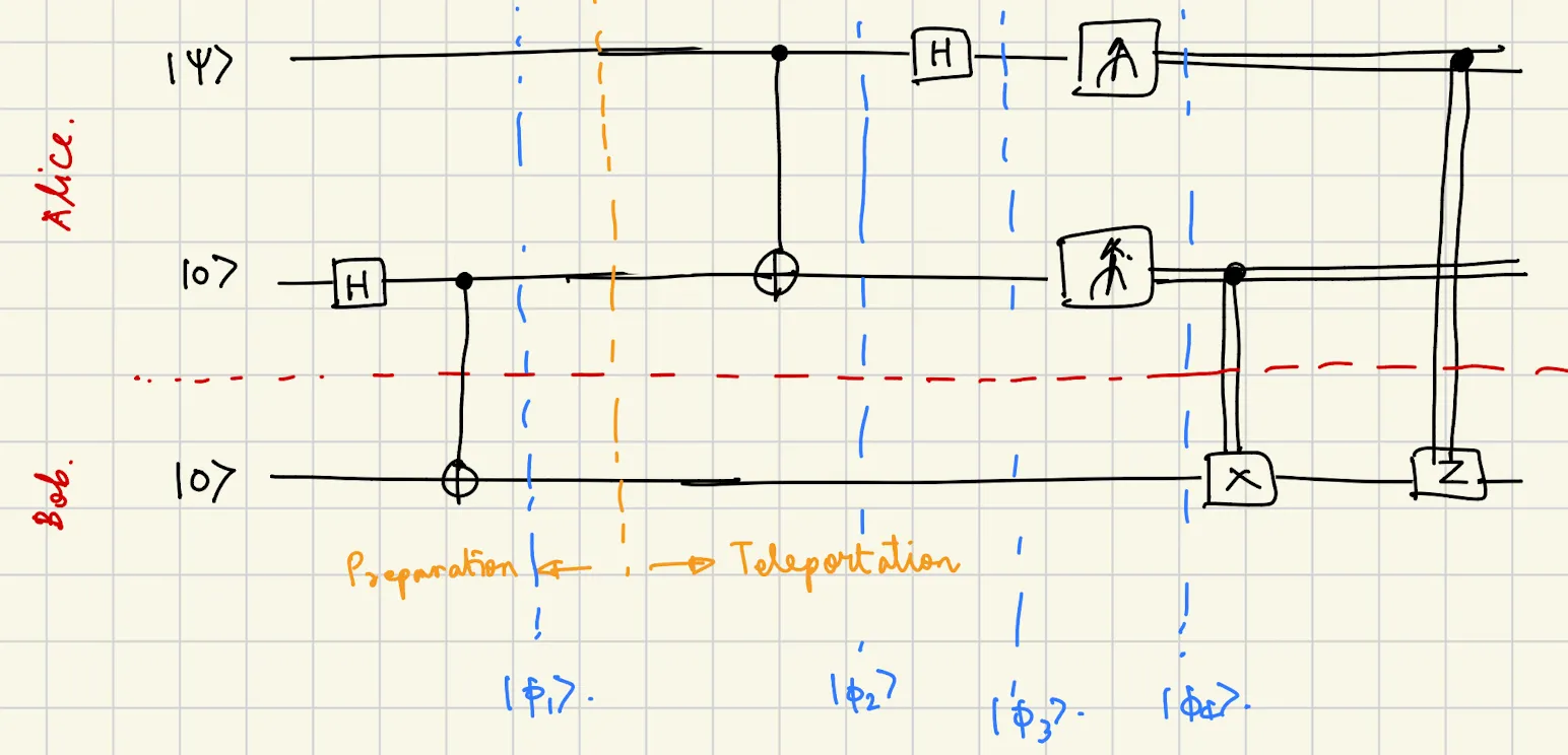
Protocol : Transfer an unknown qubit state ∣ ψ ⟩ = α ∣ 0 ⟩ + β ∣ 1 ⟩ |\psi\rangle = \alpha|0\rangle + \beta|1\rangle ∣ ψ ⟩ = α ∣0 ⟩ + β ∣1 ⟩
1 shared entangled pair (EPR pair)
2 classical bits of communication
Circuit
Step-by-Step Evolution
Initial state :
∣ ϕ 1 ⟩ = ∣ ψ ⟩ ⊗ 1 2 ( ∣ 00 ⟩ + ∣ 11 ⟩ ) |\phi_1\rangle = |\psi\rangle \otimes \frac{1}{\sqrt{2}}(|00\rangle + |11\rangle) ∣ ϕ 1 ⟩ = ∣ ψ ⟩ ⊗ 2 1 ( ∣00 ⟩ + ∣11 ⟩) Expanding ∣ ψ ⟩ = α ∣ 0 ⟩ + β ∣ 1 ⟩ |\psi\rangle = \alpha|0\rangle + \beta|1\rangle ∣ ψ ⟩ = α ∣0 ⟩ + β ∣1 ⟩
∣ ϕ 1 ⟩ = 1 2 [ α ∣ 000 ⟩ + α ∣ 011 ⟩ + β ∣ 100 ⟩ + β ∣ 111 ⟩ ] \begin{align*}
|\phi_1\rangle &= \frac{1}{\sqrt{2}}[\alpha|000\rangle + \alpha|011\rangle + \beta|100\rangle + \beta|111\rangle]
\end{align*} ∣ ϕ 1 ⟩ = 2 1 [ α ∣000 ⟩ + α ∣011 ⟩ + β ∣100 ⟩ + β ∣111 ⟩] After CNOT0 → 1 _{0\to1} 0 → 1 :
∣ ϕ 2 ⟩ = 1 2 [ α ∣ 000 ⟩ + α ∣ 011 ⟩ + β ∣ 110 ⟩ + β ∣ 101 ⟩ ] \begin{align*}
|\phi_2\rangle &= \frac{1}{\sqrt{2}}[\alpha|000\rangle + \alpha|011\rangle + \beta|110\rangle + \beta|101\rangle]
\end{align*} ∣ ϕ 2 ⟩ = 2 1 [ α ∣000 ⟩ + α ∣011 ⟩ + β ∣110 ⟩ + β ∣101 ⟩] After H on first qubit :
∣ ϕ 3 ⟩ = 1 2 [ ∣ 00 ⟩ ( α ∣ 0 ⟩ + β ∣ 1 ⟩ ) + ∣ 01 ⟩ ( α ∣ 1 ⟩ + β ∣ 0 ⟩ ) + ∣ 10 ⟩ ( α ∣ 0 ⟩ − β ∣ 1 ⟩ ) + ∣ 11 ⟩ ( α ∣ 1 ⟩ − β ∣ 0 ⟩ ) ] \begin{align*}
|\phi_3\rangle &= \frac{1}{2}\Big[|00\rangle(\alpha|0\rangle + \beta|1\rangle) + |01\rangle(\alpha|1\rangle + \beta|0\rangle) \\
&\quad\quad + |10\rangle(\alpha|0\rangle - \beta|1\rangle) + |11\rangle(\alpha|1\rangle - \beta|0\rangle)\Big]
\end{align*} ∣ ϕ 3 ⟩ = 2 1 [ ∣00 ⟩ ( α ∣0 ⟩ + β ∣1 ⟩) + ∣01 ⟩ ( α ∣1 ⟩ + β ∣0 ⟩) + ∣10 ⟩ ( α ∣0 ⟩ − β ∣1 ⟩) + ∣11 ⟩ ( α ∣1 ⟩ − β ∣0 ⟩) ] Measurement Results and Corrections
Alice measures
Bob’s state
Correction
∣ 00 ⟩ |00\rangle ∣00 ⟩ α ∣ 0 ⟩ + β ∣ 1 ⟩ \alpha|0\rangle + \beta|1\rangle α ∣0 ⟩ + β ∣1 ⟩ I I I
∣ 01 ⟩ |01\rangle ∣01 ⟩ α ∣ 1 ⟩ + β ∣ 0 ⟩ \alpha|1\rangle + \beta|0\rangle α ∣1 ⟩ + β ∣0 ⟩ X X X
∣ 10 ⟩ |10\rangle ∣10 ⟩ α ∣ 0 ⟩ − β ∣ 1 ⟩ \alpha|0\rangle - \beta|1\rangle α ∣0 ⟩ − β ∣1 ⟩ Z Z Z
∣ 11 ⟩ |11\rangle ∣11 ⟩ α ∣ 1 ⟩ − β ∣ 0 ⟩ \alpha|1\rangle - \beta|0\rangle α ∣1 ⟩ − β ∣0 ⟩ Z X ZX Z X
Result : In all cases, after Alice sends her 2 classical bits and Bob applies the appropriate correction, Bob’s qubit becomes ∣ ψ ⟩ |\psi\rangle ∣ ψ ⟩
Important :
Bob’s qubit becomes entangled with Alice’s qubits before measurement
Information about ∣ ψ ⟩ |\psi\rangle ∣ ψ ⟩
However, Bob cannot recover ∣ ψ ⟩ |\psi\rangle ∣ ψ ⟩
An n n n 2 n 2^n 2 n
∣ ψ ⟩ = ∑ x ∈ { 0 , 1 } n α x ∣ x ⟩ |\psi\rangle = \sum_{x \in \{0,1\}^n} \alpha_x|x\rangle ∣ ψ ⟩ = x ∈ { 0 , 1 } n ∑ α x ∣ x ⟩ This appears to perform 2 n 2^n 2 n
Holevo’s Theorem
Setup :
Alice has an m m m m x m_x m x
She encodes it into an n n n
Bob performs unitaries + measurement to recover m x m_x m x
Theorem : m x = m x ′ m_x = m_x' m x = m x ′ n ≥ m n \geq m n ≥ m
In other words, you need at least as many qubits as classical bits to reliably transmit information.
Superdense Coding
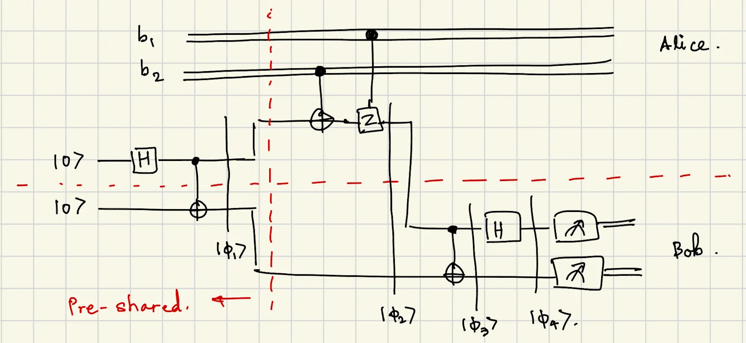
If Alice and Bob share pre-shared entanglement, then n = m / 2 n = m/2 n = m /2
Protocol : Alice can transmit 2 classical bits using 1 qubit + 1 pre-shared EPR pair.
Circuit :
Starting with EPR pair ∣ Φ 1 ⟩ = 1 2 ( ∣ 00 ⟩ + ∣ 11 ⟩ ) |\Phi_1\rangle = \frac{1}{\sqrt{2}}(|00\rangle + |11\rangle) ∣ Φ 1 ⟩ = 2 1 ( ∣00 ⟩ + ∣11 ⟩)
Alice applies gates based on ( b 1 , b 2 ) (b_1, b_2) ( b 1 , b 2 )
b 2 = 1 b_2 = 1 b 2 = 1 CNOT b 2 → 0 \text{CNOT}_{b_2\to0} CNOT b 2 → 0 b 1 = 1 b_1 = 1 b 1 = 1 C Z b 1 → 0 CZ_{b_1\to0} C Z b 1 → 0
Result: State becomes one of the four Bell states encoding b 1 b 2 b_1b_2 b 1 b 2
Bob applies CNOT + H to distinguish which Bell state, measuring ∣ b 1 b 2 ⟩ |b_1b_2\rangle ∣ b 1 b 2 ⟩
Result : 2 bits transmitted with 1 qubit!
Qubit Rotation
Consider the rotation matrix:
V θ = ( cos θ − sin θ sin θ cos θ ) V_\theta = \begin{pmatrix} \cos\theta & -\sin\theta \\ \sin\theta & \cos\theta \end{pmatrix} V θ = ( cos θ sin θ − sin θ cos θ ) This rotates a qubit ∣ ψ ⟩ |\psi\rangle ∣ ψ ⟩ θ \theta θ
Examples
For ∣ ψ ⟩ = ∣ 0 ⟩ |\psi\rangle = |0\rangle ∣ ψ ⟩ = ∣0 ⟩
V θ ∣ 0 ⟩ = ( cos θ sin θ ) V_\theta|0\rangle = \begin{pmatrix} \cos\theta \\ \sin\theta \end{pmatrix} V θ ∣0 ⟩ = ( cos θ sin θ ) For ∣ ψ ⟩ = ∣ 1 ⟩ |\psi\rangle = |1\rangle ∣ ψ ⟩ = ∣1 ⟩
V θ ∣ 1 ⟩ = ( − sin θ cos θ ) V_\theta|1\rangle = \begin{pmatrix} -\sin\theta \\ \cos\theta \end{pmatrix} V θ ∣1 ⟩ = ( − sin θ cos θ ) Rotating Two Qubits Simultaneously
( V θ ⊗ V ϕ ) ( ∣ 0 ⟩ ⊗ ∣ 0 ⟩ ) = V θ ∣ 0 ⟩ ⊗ V ϕ ∣ 0 ⟩ = ( cos θ ∣ 0 ⟩ + sin θ ∣ 1 ⟩ ) ⊗ ( cos ϕ ∣ 0 ⟩ + sin ϕ ∣ 1 ⟩ ) = cos θ cos ϕ ∣ 00 ⟩ + cos θ sin ϕ ∣ 01 ⟩ + sin θ cos ϕ ∣ 10 ⟩ + sin θ sin ϕ ∣ 11 ⟩ \begin{align*}
(V_\theta \otimes V_\phi)(|0\rangle \otimes |0\rangle) &= V_\theta|0\rangle \otimes V_\phi|0\rangle \\
&= (\cos\theta|0\rangle + \sin\theta|1\rangle) \otimes (\cos\phi|0\rangle + \sin\phi|1\rangle) \\
&= \cos\theta\cos\phi|00\rangle + \cos\theta\sin\phi|01\rangle \\
&\quad + \sin\theta\cos\phi|10\rangle + \sin\theta\sin\phi|11\rangle
\end{align*} ( V θ ⊗ V ϕ ) ( ∣0 ⟩ ⊗ ∣0 ⟩) = V θ ∣0 ⟩ ⊗ V ϕ ∣0 ⟩ = ( cos θ ∣0 ⟩ + sin θ ∣1 ⟩) ⊗ ( cos ϕ ∣0 ⟩ + sin ϕ ∣1 ⟩) = cos θ cos ϕ ∣00 ⟩ + cos θ sin ϕ ∣01 ⟩ + sin θ cos ϕ ∣10 ⟩ + sin θ sin ϕ ∣11 ⟩ Probability that first qubit is ∣ 0 ⟩ |0\rangle ∣0 ⟩
Pr [ qubit 0 is ∣ 0 ⟩ ] = cos 2 θ cos 2 ϕ + cos 2 θ sin 2 ϕ = cos 2 θ ( cos 2 ϕ + sin 2 ϕ ) = cos 2 θ \begin{align*}
\Pr[\text{qubit 0 is } |0\rangle] &= \cos^2\theta\cos^2\phi + \cos^2\theta\sin^2\phi \\
&= \cos^2\theta(\cos^2\phi + \sin^2\phi) \\
&= \cos^2\theta
\end{align*} Pr [ qubit 0 is ∣0 ⟩] = cos 2 θ cos 2 ϕ + cos 2 θ sin 2 ϕ = cos 2 θ ( cos 2 ϕ + sin 2 ϕ ) = cos 2 θ Application of Rotation: CHSH Game
The CHSH game demonstrates quantum advantage through entanglement.
Game Setup
Alice receives question x ∈ { 0 , 1 } x \in \{0,1\} x ∈ { 0 , 1 } y ∈ { 0 , 1 } y \in \{0,1\} y ∈ { 0 , 1 }
Alice responds with a ∈ { 0 , 1 } a \in \{0,1\} a ∈ { 0 , 1 } b ∈ { 0 , 1 } b \in \{0,1\} b ∈ { 0 , 1 }
Win condition : x ∧ y = a ⊕ b x \land y = a \oplus b x ∧ y = a ⊕ b
x x x y y y Win if
0
0
a = b a = b a = b
0
1
a = b a = b a = b
1
0
a = b a = b a = b
1
1
a ≠ b a \neq b a = b
Classical strategy : Maximum winning probability is 75%.
Quantum Strategy
Alice and Bob pre-share ∣ Φ + ⟩ = 1 2 ( ∣ 00 ⟩ + ∣ 11 ⟩ ) |\Phi^+\rangle = \frac{1}{\sqrt{2}}(|00\rangle + |11\rangle) ∣ Φ + ⟩ = 2 1 ( ∣00 ⟩ + ∣11 ⟩)
x x x θ A ( x ) \theta_A(x) θ A ( x ) y y y θ B ( y ) \theta_B(y) θ B ( y )
0
2 π / 8 2\pi/8 2 π /8 0
π / 8 \pi/8 π /8
1
0 0 0 1
3 π / 8 3\pi/8 3 π /8
Analysis for x = 0, y = 0
Final state after applying rotations:
∣ ψ ⟩ = ( V 2 π / 8 ⊗ V π / 8 ) ∣ Φ + ⟩ |\psi\rangle = (V_{2\pi/8} \otimes V_{\pi/8})|\Phi^+\rangle ∣ ψ ⟩ = ( V 2 π /8 ⊗ V π /8 ) ∣ Φ + ⟩ Using the identity:
cos ( θ − ϕ ) ( ∣ 00 ⟩ + ∣ 11 ⟩ ) + sin ( θ − ϕ ) ( ∣ 10 ⟩ − ∣ 01 ⟩ ) \cos(\theta - \phi)(|00\rangle + |11\rangle) + \sin(\theta - \phi)(|10\rangle - |01\rangle) cos ( θ − ϕ ) ( ∣00 ⟩ + ∣11 ⟩) + sin ( θ − ϕ ) ( ∣10 ⟩ − ∣01 ⟩) For θ = 2 π / 8 , ϕ = π / 8 \theta = 2\pi/8, \phi = \pi/8 θ = 2 π /8 , ϕ = π /8
Pr [ qubit 0 is ∣ 0 ⟩ ] = cos 2 ( π / 8 ) ≈ 0.8534 \Pr[\text{qubit 0 is } |0\rangle] = \cos^2(\pi/8) \approx 0.8534 Pr [ qubit 0 is ∣0 ⟩] = cos 2 ( π /8 ) ≈ 0.8534 Similarly, for x = 1 , y = 1 x=1, y=1 x = 1 , y = 1
Pr [ qubit 0 is ∣ 1 ⟩ ] = sin 2 ( π / 8 ) = cos 2 ( − π / 8 ) ≈ 0.8534 \Pr[\text{qubit 0 is } |1\rangle] = \sin^2(\pi/8) = \cos^2(-\pi/8) \approx 0.8534 Pr [ qubit 0 is ∣1 ⟩] = sin 2 ( π /8 ) = cos 2 ( − π /8 ) ≈ 0.8534 Overall winning probability : ≈ 85.4 % \approx 85.4\% ≈ 85.4%
Universal Gate Sets
A gate set G \mathcal{G} G universal if for any unitary U U U G \mathcal{G} G approximate U U U
U U U ϵ \epsilon ϵ V V V ∣ ψ ⟩ |\psi\rangle ∣ ψ ⟩
∥ U ∣ ψ ⟩ − V ∣ ψ ⟩ ∥ ≤ ϵ \|U|\psi\rangle - V|\psi\rangle\| \leq \epsilon ∥ U ∣ ψ ⟩ − V ∣ ψ ⟩ ∥ ≤ ϵ Any circuit C C C
Example 1: Continuous Rotations + Phase Shift
R x ( θ ) = ( cos θ − i sin θ − i sin θ cos θ ) R y ( θ ) = ( cos θ − sin θ sin θ cos θ ) R z ( θ ) = ( e − i θ 0 0 e i θ ) P ( θ ) = ( 1 0 0 e i θ ) \begin{align*}
R_x(\theta) &= \begin{pmatrix} \cos\theta & -i\sin\theta \\ -i\sin\theta & \cos\theta \end{pmatrix} \\[1em]
R_y(\theta) &= \begin{pmatrix} \cos\theta & -\sin\theta \\ \sin\theta & \cos\theta \end{pmatrix} \\[1em]
R_z(\theta) &= \begin{pmatrix} e^{-i\theta} & 0 \\ 0 & e^{i\theta} \end{pmatrix} \\[1em]
P(\theta) &= \begin{pmatrix} 1 & 0 \\ 0 & e^{i\theta} \end{pmatrix}
\end{align*} R x ( θ ) R y ( θ ) R z ( θ ) P ( θ ) = ( cos θ − i sin θ − i sin θ cos θ ) = ( cos θ sin θ − sin θ cos θ ) = ( e − i θ 0 0 e i θ ) = ( 1 0 0 e i θ ) These must work for all 0 ≤ θ < 2 π 0 \leq \theta < 2\pi 0 ≤ θ < 2 π
Note : Both examples require at least one 2-qubit gate (CNOT).
Example 2: Discrete + Finite Gates
H = 1 2 ( 1 1 1 − 1 ) CNOT (2-qubit gate) S = ( 1 0 0 i ) T = ( 1 0 0 e i π / 4 ) \begin{align*}
H &= \frac{1}{\sqrt{2}}\begin{pmatrix} 1 & 1 \\ 1 & -1 \end{pmatrix} \\[1em]
\text{CNOT} &\text{ (2-qubit gate)} \\[1em]
S &= \begin{pmatrix} 1 & 0 \\ 0 & i \end{pmatrix} \\[1em]
T &= \begin{pmatrix} 1 & 0 \\ 0 & e^{i\pi/4} \end{pmatrix}
\end{align*} H CNOT S T = 2 1 ( 1 1 1 − 1 ) (2-qubit gate) = ( 1 0 0 i ) = ( 1 0 0 e iπ /4 ) Deutsch’s Algorithm
Problem : Given oracle access to f : { 0 , 1 } → { 0 , 1 } f: \{0,1\} \to \{0,1\} f : { 0 , 1 } → { 0 , 1 } f ( 0 ) = f ( 1 ) f(0) = f(1) f ( 0 ) = f ( 1 )
Classical : Any classical algorithm needs to query f f f 2 times .
Quantum : Deutsch’s algorithm uses only 1 query !
Quantum Oracle
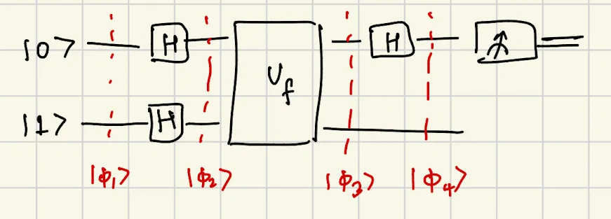
A quantum circuit accesses f f f
U f ∣ x , b ⟩ = ∣ x , b ⊕ f ( x ) ⟩ U_f|x,b\rangle = |x, b \oplus f(x)\rangle U f ∣ x , b ⟩ = ∣ x , b ⊕ f ( x )⟩ Circuit
Analysis
∣ ϕ 1 ⟩ = ∣ 0 ⟩ ∣ 1 ⟩ ∣ ϕ 2 ⟩ = ∣ + ⟩ ∣ − ⟩ = 1 2 ( ∣ 00 ⟩ − ∣ 01 ⟩ + ∣ 10 ⟩ − ∣ 11 ⟩ ) \begin{align*}
|\phi_1\rangle &= |0\rangle|1\rangle \\[0.5em]
|\phi_2\rangle &= |+\rangle|-\rangle = \frac{1}{2}(|00\rangle - |01\rangle + |10\rangle - |11\rangle)
\end{align*} ∣ ϕ 1 ⟩ ∣ ϕ 2 ⟩ = ∣0 ⟩ ∣1 ⟩ = ∣ + ⟩ ∣ − ⟩ = 2 1 ( ∣00 ⟩ − ∣01 ⟩ + ∣10 ⟩ − ∣11 ⟩) After U f U_f U f
∣ ϕ 3 ⟩ = 1 2 [ ∣ 0 , f ( 0 ) ⟩ − ∣ 0 , f ( 0 ) ‾ ⟩ + ∣ 1 , f ( 1 ) ⟩ − ∣ 1 , f ( 1 ) ‾ ⟩ ] \begin{align*}
|\phi_3\rangle &= \frac{1}{2}[|0,f(0)\rangle - |0,\overline{f(0)}\rangle + |1,f(1)\rangle - |1,\overline{f(1)}\rangle]
\end{align*} ∣ ϕ 3 ⟩ = 2 1 [ ∣0 , f ( 0 )⟩ − ∣0 , f ( 0 ) ⟩ + ∣1 , f ( 1 )⟩ − ∣1 , f ( 1 ) ⟩] Using ∣ b ⟩ − ∣ b ˉ ⟩ = ( X b ∣ − ⟩ ) |b\rangle - |\bar{b}\rangle = (X^b|-\rangle) ∣ b ⟩ − ∣ b ˉ ⟩ = ( X b ∣ − ⟩)
∣ ϕ 3 ⟩ = 1 2 ( ∣ 0 ⟩ X f ( 0 ) + ∣ 1 ⟩ X f ( 1 ) ) ∣ − ⟩ |\phi_3\rangle = \frac{1}{\sqrt{2}}(|0\rangle X^{f(0)} + |1\rangle X^{f(1)})|-\rangle ∣ ϕ 3 ⟩ = 2 1 ( ∣0 ⟩ X f ( 0 ) + ∣1 ⟩ X f ( 1 ) ) ∣ − ⟩ After Hadamard on first qubit:
∣ ϕ 4 ⟩ = 1 2 [ ( ∣ 0 ⟩ + ∣ 1 ⟩ ) X f ( 0 ) + ( ∣ 0 ⟩ − ∣ 1 ⟩ ) X f ( 1 ) ] ∣ − ⟩ |\phi_4\rangle = \frac{1}{2}[(|0\rangle + |1\rangle)X^{f(0)} + (|0\rangle - |1\rangle)X^{f(1)}]|-\rangle ∣ ϕ 4 ⟩ = 2 1 [( ∣0 ⟩ + ∣1 ⟩) X f ( 0 ) + ( ∣0 ⟩ − ∣1 ⟩) X f ( 1 ) ] ∣ − ⟩ Result : The first qubit becomes:
First qubit = { ∣ 0 ⟩ if f ( 0 ) = f ( 1 ) (constant function) ∣ 1 ⟩ if f ( 0 ) ≠ f ( 1 ) (balanced function) \text{First qubit} = \begin{cases}
|0\rangle & \text{if } f(0) = f(1) \text{ (constant function)} \\
|1\rangle & \text{if } f(0) \neq f(1) \text{ (balanced function)}
\end{cases} First qubit = { ∣0 ⟩ ∣1 ⟩ if f ( 0 ) = f ( 1 ) (constant function) if f ( 0 ) = f ( 1 ) (balanced function) Conclusion : Measure the first qubit to distinguish the cases with 1 query!
Phase Kickback
Phase kickback is a key phenomenon where the phase from the target qubit “kicks back” to the control register.
General Principle
For operator X X X
∣ b ⊕ c ⟩ = X c ∣ b ⟩ |b \oplus c\rangle = X^c|b\rangle ∣ b ⊕ c ⟩ = X c ∣ b ⟩ Therefore:
U f ( ∣ b ⟩ ∣ a ⟩ ) = ∣ b ⟩ ∣ a ⊕ f ( b ) ⟩ = ∣ b ⟩ ( X f ( b ) ∣ a ⟩ ) U_f(|b\rangle|a\rangle) = |b\rangle|a \oplus f(b)\rangle = |b\rangle(X^{f(b)}|a\rangle) U f ( ∣ b ⟩ ∣ a ⟩) = ∣ b ⟩ ∣ a ⊕ f ( b )⟩ = ∣ b ⟩ ( X f ( b ) ∣ a ⟩) By linearity, this holds for all quantum states ∣ ψ ⟩ = ∑ i ∣ i ⟩ |\psi\rangle = \sum_i |i\rangle ∣ ψ ⟩ = ∑ i ∣ i ⟩
U f ( ∣ b ⟩ ∣ ψ ⟩ ) = ∣ b ⟩ ( X f ( b ) ∣ ψ ⟩ ) U_f(|b\rangle|\psi\rangle) = |b\rangle(X^{f(b)}|\psi\rangle) U f ( ∣ b ⟩ ∣ ψ ⟩) = ∣ b ⟩ ( X f ( b ) ∣ ψ ⟩) Application in Deutsch’s Algorithm
In Deutsch’s problem with target qubit in ∣ − ⟩ |-\rangle ∣ − ⟩
U f ( ∣ + ⟩ ∣ − ⟩ ) = 1 2 [ U f ( ∣ 0 ⟩ ∣ − ⟩ ) + U f ( ∣ 1 ⟩ ∣ − ⟩ ) ] = 1 2 [ ∣ 0 ⟩ X f ( 0 ) ∣ − ⟩ + ∣ 1 ⟩ X f ( 1 ) ∣ − ⟩ ] \begin{align*}
U_f(|+\rangle|-\rangle) &= \frac{1}{\sqrt{2}}[U_f(|0\rangle|-\rangle) + U_f(|1\rangle|-\rangle)] \\
&= \frac{1}{\sqrt{2}}[|0\rangle X^{f(0)}|-\rangle + |1\rangle X^{f(1)}|-\rangle]
\end{align*} U f ( ∣ + ⟩ ∣ − ⟩) = 2 1 [ U f ( ∣0 ⟩ ∣ − ⟩) + U f ( ∣1 ⟩ ∣ − ⟩)] = 2 1 [ ∣0 ⟩ X f ( 0 ) ∣ − ⟩ + ∣1 ⟩ X f ( 1 ) ∣ − ⟩] Since X ∣ − ⟩ = − ∣ − ⟩ X|-\rangle = -|-\rangle X ∣ − ⟩ = − ∣ − ⟩ X ∣ + ⟩ = ∣ + ⟩ X|+\rangle = |+\rangle X ∣ + ⟩ = ∣ + ⟩
X 0 ∣ − ⟩ = ∣ − ⟩ X 1 ∣ − ⟩ = − ∣ − ⟩ \begin{align*}
X^0|-\rangle &= |-\rangle \\
X^1|-\rangle &= -|-\rangle
\end{align*} X 0 ∣ − ⟩ X 1 ∣ − ⟩ = ∣ − ⟩ = − ∣ − ⟩ Thus the global phase depends on f f f
H ∣ a ⟩ = 1 2 ∑ b ∈ { 0 , 1 } ( − 1 ) a b ∣ b ⟩ H|a\rangle = \frac{1}{\sqrt{2}}\sum_{b \in \{0,1\}} (-1)^{ab}|b\rangle H ∣ a ⟩ = 2 1 b ∈ { 0 , 1 } ∑ ( − 1 ) ab ∣ b ⟩ Multi-Qubit Hadamard
Applying H H H n n n
H ⊗ n ∣ x 0 … x n − 1 ⟩ = H ∣ x 0 ⟩ ⊗ H ∣ x 1 ⟩ ⊗ ⋯ ⊗ H ∣ x n − 1 ⟩ = ( 1 2 ∑ b 0 ( − 1 ) x 0 b 0 ∣ b 0 ⟩ ) ⊗ ( 1 2 ∑ b 1 ( − 1 ) x 1 b 1 ∣ b 1 ⟩ ) ⊗ ⋯ = 1 2 n ∑ y ∈ { 0 , 1 } n ( − 1 ) x ⋅ y ∣ y ⟩ \begin{align*}
H^{\otimes n}|x_0\ldots x_{n-1}\rangle &= H|x_0\rangle \otimes H|x_1\rangle \otimes \cdots \otimes H|x_{n-1}\rangle \\
&= \left(\frac{1}{\sqrt{2}}\sum_{b_0}(-1)^{x_0 b_0}|b_0\rangle\right) \otimes \left(\frac{1}{\sqrt{2}}\sum_{b_1}(-1)^{x_1 b_1}|b_1\rangle\right) \otimes \cdots \\
&= \frac{1}{\sqrt{2^n}}\sum_{y \in \{0,1\}^n} (-1)^{x \cdot y}|y\rangle
\end{align*} H ⊗ n ∣ x 0 … x n − 1 ⟩ = H ∣ x 0 ⟩ ⊗ H ∣ x 1 ⟩ ⊗ ⋯ ⊗ H ∣ x n − 1 ⟩ = ( 2 1 b 0 ∑ ( − 1 ) x 0 b 0 ∣ b 0 ⟩ ) ⊗ ( 2 1 b 1 ∑ ( − 1 ) x 1 b 1 ∣ b 1 ⟩ ) ⊗ ⋯ = 2 n 1 y ∈ { 0 , 1 } n ∑ ( − 1 ) x ⋅ y ∣ y ⟩ where x ⋅ y = x 0 y 0 ⊕ x 1 y 1 ⊕ ⋯ ⊕ x n − 1 y n − 1 x \cdot y = x_0y_0 \oplus x_1y_1 \oplus \cdots \oplus x_{n-1}y_{n-1} x ⋅ y = x 0 y 0 ⊕ x 1 y 1 ⊕ ⋯ ⊕ x n − 1 y n − 1
Key Result
H ⊗ n ∣ x ⟩ = 1 2 n ∑ y ∈ { 0 , 1 } n ( − 1 ) x ⋅ y ∣ y ⟩ H^{\otimes n}|x\rangle = \frac{1}{\sqrt{2^n}}\sum_{y \in \{0,1\}^n} (-1)^{x \cdot y}|y\rangle H ⊗ n ∣ x ⟩ = 2 n 1 y ∈ { 0 , 1 } n ∑ ( − 1 ) x ⋅ y ∣ y ⟩ This creates an equal superposition over all 2 n 2^n 2 n x ⋅ y x \cdot y x ⋅ y
Simons’ Algorithm
Problem : Given oracle access to f : { 0 , 1 } n → { 0 , 1 } n f: \{0,1\}^n \to \{0,1\}^n f : { 0 , 1 } n → { 0 , 1 } n s ∈ { 0 , 1 } n s \in \{0,1\}^n s ∈ { 0 , 1 } n
f ( x ) = f ( y ) ⟺ x ⊕ y = s f(x) = f(y) \iff x \oplus y = s f ( x ) = f ( y ) ⟺ x ⊕ y = s Find the hidden string s s s
Classical complexity : O ( 2 n / 2 ) O(2^{n/2}) O ( 2 n /2 )
Quantum complexity : O ( n ) O(n) O ( n )
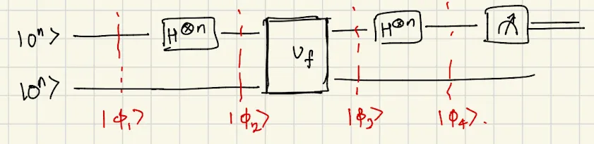
Simons’ Quantum Subroutine
Circuit queries U f U_f U f y ∈ { 0 , 1 } n y \in \{0,1\}^n y ∈ { 0 , 1 } n s ⋅ y = 0 s \cdot y = 0 s ⋅ y = 0
Analysis
∣ ϕ 1 ⟩ = ∣ 0 n ⟩ ⊗ ∣ 0 n ⟩ ∣ ϕ 2 ⟩ = ( 1 2 n ∑ x ∈ { 0 , 1 } n ∣ x ⟩ ) ⊗ ∣ 0 n ⟩ \begin{align*}
|\phi_1\rangle &= |0^n\rangle \otimes |0^n\rangle \\[0.5em]
|\phi_2\rangle &= \left(\frac{1}{\sqrt{2^n}}\sum_{x \in \{0,1\}^n}|x\rangle\right) \otimes |0^n\rangle
\end{align*} ∣ ϕ 1 ⟩ ∣ ϕ 2 ⟩ = ∣ 0 n ⟩ ⊗ ∣ 0 n ⟩ = 2 n 1 x ∈ { 0 , 1 } n ∑ ∣ x ⟩ ⊗ ∣ 0 n ⟩ After U f U_f U f
∣ ϕ 3 ⟩ = 1 2 n ∑ x ∈ { 0 , 1 } n ∣ x ⟩ ⊗ ∣ f ( x ) ⟩ \begin{align*}
|\phi_3\rangle &= \frac{1}{\sqrt{2^n}}\sum_{x \in \{0,1\}^n}|x\rangle \otimes |f(x)\rangle
\end{align*} ∣ ϕ 3 ⟩ = 2 n 1 x ∈ { 0 , 1 } n ∑ ∣ x ⟩ ⊗ ∣ f ( x )⟩ Suppose we measure the second register and get outcome a a a x x x f ( x ) = a f(x) = a f ( x ) = a
By the promise, there are exactly two such values: x a x_a x a x a ⊕ s x_a \oplus s x a ⊕ s
1 2 ( ∣ x a ⟩ + ∣ x a ⊕ s ⟩ ) ⊗ ∣ a ⟩ \frac{1}{\sqrt{2}}(|x_a\rangle + |x_a \oplus s\rangle) \otimes |a\rangle 2 1 ( ∣ x a ⟩ + ∣ x a ⊕ s ⟩) ⊗ ∣ a ⟩ After applying H ⊗ n H^{\otimes n} H ⊗ n
∣ ϕ 4 ⟩ = 1 2 n + 1 ∑ y ∈ { 0 , 1 } n [ ( − 1 ) x a ⋅ y + ( − 1 ) ( x a ⊕ s ) ⋅ y ] ∣ y ⟩ ∣ a ⟩ \begin{align*}
|\phi_4\rangle &= \frac{1}{\sqrt{2^{n+1}}}\sum_{y \in \{0,1\}^n}\left[(-1)^{x_a \cdot y} + (-1)^{(x_a \oplus s) \cdot y}\right]|y\rangle|a\rangle
\end{align*} ∣ ϕ 4 ⟩ = 2 n + 1 1 y ∈ { 0 , 1 } n ∑ [ ( − 1 ) x a ⋅ y + ( − 1 ) ( x a ⊕ s ) ⋅ y ] ∣ y ⟩ ∣ a ⟩ Using ( x a ⊕ s ) ⋅ y = x a ⋅ y ⊕ s ⋅ y (x_a \oplus s) \cdot y = x_a \cdot y \oplus s \cdot y ( x a ⊕ s ) ⋅ y = x a ⋅ y ⊕ s ⋅ y
∣ ϕ 4 ⟩ = 1 2 n + 1 ∑ y ∈ { 0 , 1 } n ( − 1 ) x a ⋅ y [ 1 + ( − 1 ) s ⋅ y ] ∣ y ⟩ ∣ a ⟩ \begin{align*}
|\phi_4\rangle &= \frac{1}{\sqrt{2^{n+1}}}\sum_{y \in \{0,1\}^n}(-1)^{x_a \cdot y}\left[1 + (-1)^{s \cdot y}\right]|y\rangle|a\rangle
\end{align*} ∣ ϕ 4 ⟩ = 2 n + 1 1 y ∈ { 0 , 1 } n ∑ ( − 1 ) x a ⋅ y [ 1 + ( − 1 ) s ⋅ y ] ∣ y ⟩ ∣ a ⟩ Key observation : The coefficient 1 + ( − 1 ) s ⋅ y 1 + (-1)^{s \cdot y} 1 + ( − 1 ) s ⋅ y
1 + ( − 1 ) s ⋅ y = { 2 if s ⋅ y = 0 (constructive interference) 0 if s ⋅ y = 1 (destructive interference) 1 + (-1)^{s \cdot y} = \begin{cases}
2 & \text{if } s \cdot y = 0 \text{ (constructive interference)} \\
0 & \text{if } s \cdot y = 1 \text{ (destructive interference)}
\end{cases} 1 + ( − 1 ) s ⋅ y = { 2 0 if s ⋅ y = 0 (constructive interference) if s ⋅ y = 1 (destructive interference) Therefore, measuring y y y y y y s ⋅ y = 0 s \cdot y = 0 s ⋅ y = 0
Classical Post-Processing
After obtaining m = O ( n ) m = O(n) m = O ( n ) y ( 1 ) , y ( 2 ) , … , y ( m ) y^{(1)}, y^{(2)}, \ldots, y^{(m)} y ( 1 ) , y ( 2 ) , … , y ( m )
y ( 1 ) ⋅ s = 0 y ( 2 ) ⋅ s = 0 ⋮ y ( m ) ⋅ s = 0 \begin{align*}
y^{(1)} \cdot s &= 0 \\
y^{(2)} \cdot s &= 0 \\
&\vdots \\
y^{(m)} \cdot s &= 0
\end{align*} y ( 1 ) ⋅ s y ( 2 ) ⋅ s y ( m ) ⋅ s = 0 = 0 ⋮ = 0 This is a system of linear equations over F 2 \mathbb{F}_2 F 2 O ( n 3 ) O(n^3) O ( n 3 )
Result : Simons’ algorithm finds s s s
Further Topics
TBD:
Quantum Fourier Transform
Quantum Phase Estimation
Shor’s Factoring Algorithm
Grover’s Search and Quantum Counting
Quantum Error Correction
Quantum Complexity Theory